When it comes to archaeological photography, capturing the best possible images, whether of small artifacts or large sites, requires thoughtful Read more
The Thornborough Henges are located within a distinctive and complex landscape that has been shaped over millennia by a combination Read more
Introduction to the European Ice Age
What Is an “Ice Age”?
In geological terms an Ice Age is a multi‑million‑year interval during which permanent ice sheets persist at one or both poles. Within an ice age the climate oscillates between cold glacial stages—when ice expands far from its cores—and warmer interglacials like our present Holocene. We live inside the Quaternary Ice Age (2.6 Ma–present); the “Last Ice Age” that concerns archaeology is the most recent glacial cycle of this longer icy era.
A Brief History of Ice Ages on Earth
Geological era
Major ice ages
Key drivers
2.4–2.1 Ga
Huronian
Rising oxygen + continental positions
720–635 Ma
Cryogenian (“Snowball Earth”)
Albedo feedback during Rodinia breakup
450–420 Ma
Late Ordovician–Silurian
Gondwana at the South Pole + CO₂ draw‑down
360–260 Ma
Carboniferous–Permian
Mountain uplift, coal swamp carbon burial
34 Ma–present
Cenozoic / Quaternary
Antarctic isolation, Himalayan uplift, orbital forcing
Within the Quaternary at least 11 full glacial–interglacial cycles are recognised, paced by Milanković orbital parameters (eccentricity 100 ka, obliquity 41 ka, precession 23 ka) that modulate high‑latitude summer insolation.
Neanderthal skulls
Human Storylines in Ice‑Age Europe
Early hominins (Homo antecessor at Atapuerca > 1 Ma) arrived during a temperate window.
Neanderthals survived multiple glacial periods but retreated to southern refugia by the Last Glacial Maximum (LGM).
Homo sapiens entered c. 45 ka, endured MIS‑3 climatic whiplash, then recolonised deglaciated Northern Europe after 15 ka.
Each cold phase fragmented habitat and opened or closed migration corridors—a framework vital to our Brigantian questions.
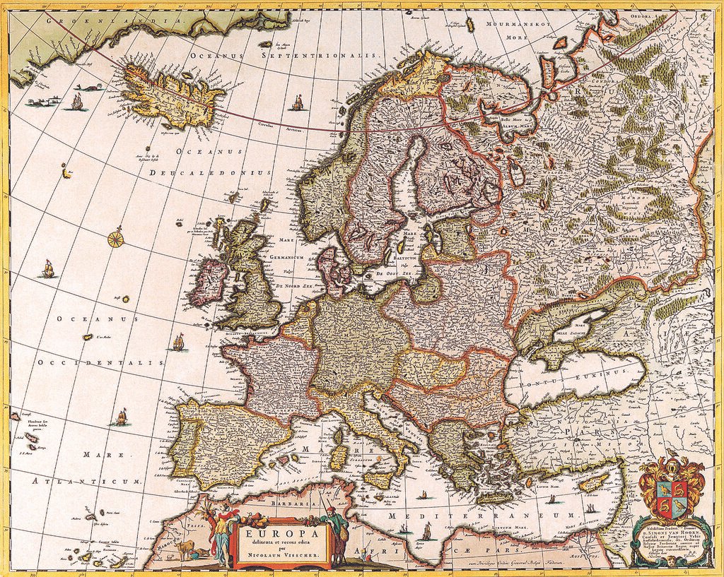
The Last Glacial Cycle in Europe (115 ka – 11.7 ka)
Western Britain: Welsh & Cumbrian glaciers fed an Irish‑Sea ice lobe; retreat formed proglacial lakes and east‑coast routes.
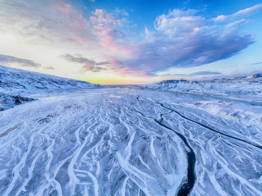
North‑Sea Plain:Periglacial Doggerland linked Britain to Continent until c. 8 ka.
Central Europe & Baltic: Scandinavian ice carved Moraines south of Berlin–Warsaw; meltwaters birthed Oder & Vistula.
Alpine & Carpathians: Glacier tongues dammed lakes; Danube corridor remained a key east–west passage.
Why This Matters for Our Programme
Migration Gateways – Timing of the Atlantic, Doggerland and Danubian corridors underpins models for Brigantian and other tribal movements.
Population Bottlenecks – Genetic Drift in refugia helps explain later Iron‑Age tribal discontinuities.
Technological Pulses – Cold‑phase compression followed by warming often coincides with innovations (microliths, archery).
Forthcoming country chapters will layer this glacial template onto local pollen, sea‑level and archaeological datasets—from Galicia’s bays to the Baltic morainic arcs—building a high‑resolution atlas of human resilience and mobility across Ice‑Age Europe.
<H3 data-pm-slice="1 1 []">How Do Ice Ages Form—and Where Do Ice Sheets Grow?
The Cooling Mechanisms
Orbital (Milanković) Cycles – Quasi‑periodic variations in Earth’s orbit change summer solar input at high latitudes. If boreal summers grow too cool, winter snow survives and the high‑albedo surface reflects more sunlight, amplifying the chill.
Greenhouse‑Gas Dips – Long‑term tectonic or biological sequestration of CO₂/CH₄ thins the atmospheric “duvet,” letting more heat radiate to space.
Tectonic & Oceanic Rearrangements – Continental drift can place land over poles (permitting vast ice sheets) or reroute warm currents (e.g., closure of Central American Seaway strengthened Atlantic meridional overturning and intensified high‑latitude snowfall).
Volcanic & Dust Feedbacks – Major eruptions and continental‑scale dust storms boost stratospheric aerosols, shading the planet and nurturing further snowpack.
Geographic Controls on Ice Distribution
Factor
Effect
European expression
Latitude
Low summer sun northward of 60 ° N favours year‑round snow
Fennoscandian & British‑Irish domes nucleated above 60 ° N and radiated outward
Altitude
Cooler air aloft lowers the Equilibrium Line Altitude (ELA)
Alps, Pyrenees and Scottish Highlands held valley glaciers even at 45–57 ° N
Continentality
Interior regions with low winter humidity may remain ice‑free despite cold
Eastern European Plain south of Moscow saw patchy Loess but little ice
Proximity to Moisture
Maritime areas with heavy snowfall build thick ice despite milder temps
Norwegian Atlantic façade and western Scotland developed extensive névé zones
Thus, ice thickness declines equator‑ward, but high‑relief coastal zones can rival polar deposits, while dry continental basins may remain periglacial rather than glaciated.
Planet Under Ice — The Consequences of a Colder World
Geological Transformation
Process
Resulting landforms
Examples across West‑to‑Baltic Europe
Glacial Erosion
U‑shaped valleys, fjords, corries
Hardangerfjord (Norway), Glencoe (Scotland), Val d’Anniviers (Alps)
Abrasion & Plucking
Striated bedrock, roche moutonnées
Lake District scarps, Bohuslän archipelago
Deposition
Moraines, Drumlins, eskers, till plains
Yorkshire Vale Drumlin swarm, Saalian push moraines in Poland
Isostatic rebound
Raised beaches, marine terraces
Scotland’s “Parallel Roads” of Glen Roy; Baltic Sea strandlines
Meltwater Megafloods
Outburst channels, loess blankets
Channel River spillway (Channel Isles), Pripet Marsh silt fans
Glaciation therefore creates topographic diversity and redirects drainage: proglacial lakes dammed by ice and debris can breach, carving spillways that later guide human routeways (e.g., Tyne–Solway gap; Øresund).
Impact on Ecosystems & Resources
Domain
Ice‑age response
Knock‑on effects
Flora
Boreal steppe‑tundra replaced temperate forest north of ~47 ° N; refugia persisted in Iberia, Italy, Balkans
Source areas for post‑glacial tree recolonisation; today’s genetic hotspots (e.g., Iberian oaks)
Possible landscape engravings on plaquettes from Les Varines, Jersey
Social risk
Long‑distance exchange networks for exogamy & obsidian/flint
Exotic raw‑material sourcing >300 km (Solutrean Corbières flint at Montlleó)
Technological leaps
Pressure‑flaking microblades, atlatl, bow
Early bow fragments in Holmegård, Denmark; Solutrean laurel‑leaf bifaces
From Survival to Flourishing
Despite harsh climates, population rebounds after 20 ka show successful adaptation. Art (Lascaux, Altamira), complex burial rites (Sunghir), and large aggregation sites (Pavlov) testify that culture flowered, not merely endured. These technological and social innovations laid foundations for Mesolithic exploitation of post‑glacial environments—and for later tribal identities such as the Brigantes.
Upcoming chapters will unpack these adaptive strategy’s region‑by‑region, tracing how glacial legacies shaped ecological niches, resource frontiers, and the cultural mosaics into which our target populations emerged.
Zoning the Chill — A Spectrum of Glacial Harshness
We can now introduce the idea of glacial “zones” of harshness – we need to try to map a spectrum of zones of harshness over time, and covering the land and sea masses of Europe. We would need to understand how the local geography, nature, and humanity would respond to that. For example, hardness of rock, direction of existing valleys, Solar variances, altitude, etc. We can mention our core timeline of interest is from the Palaeolithic period onwards.
Concept of “Harshness Zones”
Rather than a single snow‑line, a European ice age generated concentric or patchy bands of severity determined by latitude, altitude, bedrock, oceanicity and solar aspect. Each zone imposed distinctive constraints and opportunities on landscapes, ecosystems and humans.
Zone label
Typical LGM climate
Key physical drivers
Representative terrain
Biotic & human implications
Core Ice‑Dome
Permanent ice cap, ‑30 °C mean annual
High latitude/altitude; positive mass balance
Scandinavian shield, Ben Nevis plateau
Uninhabitable; glacial scouring creates raw mineral surfaces for post‑glacial soils
Polar Desert
Sparse snow, fierce katabatic winds, permafrost
Rain‑shadow lee of domes; low moisture
Doggerland interior, southern North Sea plain
Patchy steppe; limited wood; humans visit seasonally for reindeer drives
Periglacial Steppe
Long winters < ‑15 °C; brief 10 °C summer
Distance from westerlies; loess deposition
Hungarian Plain margins, Champagne chalklands
Rich grazing → mammoth/reindeer herds; seasonally mobile hunters
Montane Valley Glaciation
Glacier tongues fill troughs; refugia on sunny slopes
Altitude + orographic snow
Alps, Pyrenees, Scottish Highlands
Ecological “islands” for endemics; humans exploit rock‑shelters above ice
Temperate Refugia
Mean annual > 5 °C; mixed forest pockets
Low latitude, maritime influence, rain‑shadow
Cantabrian coast, Rhône corridor, Po valley
Continuous human occupation; seed banks for post‑glacial biota
Bølling–Allerød (14.7–12.9 ka): Polar desert retracts to Baltic rim; temperate refugia expand north of 50 °N. Hunter networks fuse, fostering Magdalenian art fluorescence.
Younger Dryas (12.9–11.7 ka): Bands snap southward ~500 km within decades. Human groups contract to Atlantic façade and Carpathian foothills; techno‑systems simplify (Federmesser).
Early Holocene (11.7–8 ka): Core ice retreats to Scandinavia; periglacial steppe replaced by birch–pine parkland; maritime shelf fringe drowns (Doggerland diaspora).
“Harshness Modifiers” — Local Factors
Modifier
Amplifies or buffers cold?
Illustration
Rock Hardness
Tough gneiss/granite resists scour, leaving high Tors; soft chalk erodes into dry valleys
Granite tors of Bodmin Moor remained nunataks above valley ice
Valley Orientation
Troughs aligned to ice flow funnel glaciers; transverse valleys form lee refugia
East–west Welsh valleys glaciated deeply; north‑facing side‑glen at Cwm Idwal held early post‑glacial flora
Interiors lacked snowfall, moderating ice build; coasts got heavy snow but warmer winters
East Baltic interior periglacial dune fields vs. Norwegian fjord full‑thickness ice
Ocean Current Variability
North Atlantic meltwater pulses stalled AMOC, deepening chill on NW Europe
Heinrich‑1 outburst 17 ka thickened Irish Sea lobe
Implications for Our Research Agenda
Route Viability Modelling – Incorporate zone maps into least‑cost path models for Late‑Glacial migrations.
Refugium Genetics – Target aDNA sampling in refugia pockets (Cantabria, Garonne, Alps) to capture founder lineages.
Geo‑archaeological Coring – Multi‑proxy lake cores at zone margins track biotic turnover and human signal intensity.
Rock Shelter Survey Bias – Recognise survey gaps in lee‑side refugia valleys that may hide continuous occupation sequences crucial for understanding Brigantian origins.
Mapping harshness spectra through time converts “ice maps” into dynamic habitat and mobility surfaces—essential for reconstructing how ancestors navigated, settled, and eventually formed the confederations we now seek to trace.
Mapping Erosion Intensity vs. Local Geology
To operationalise these zones we propose a geo‑morpho‑lithic overlay: plotting characteristic glacial landforms against a resistance index for underlying bedrock and regolith. This cross‑comparison helps grade landscapes by impact severity—from “scoured raw” to “lightly frost‑shattered.”
Data layer
Metric / proxy
Why it matters
Example application
Landform inventory
Digital mapping of drumlins, roches moutonnées, meltwater channels, block‑fields
The density and scale of erosion/deposition features mirror the mechanical power of the ice
Rock strength classes (UCS, fracture density), weathering index
Hard rocks (granite, gneiss) yield dramatic whalebacks; weak mudstones become streamlined low drumlins
Compare Scottish Benbulben sandstone benches with Norwegian gneiss trough‑walls
Thermo‑dynamic regime
Modelling freeze–thaw cycles, permafrost depth
In temperate margins sub‑glacial meltwater and seasonal frost drive quarry‑like fragmentation
Periglacial tors on Dartmoor vs. polish on Scandinavian shield
Slope & aspect
DEM‑derived insolation and stress fields
South‑facing slopes in mid‑latitudes thaw faster, enhancing block‑field creep rather than abrasion
Asymmetric valley profiles in Pyrenees record sun‑exposed debris fans
Palaeo‑ice dynamics
Flow velocity reconstructions from lineations
Faster ice = more abrasive power where bedrock permits
Irish Sea lobe lineations tie to soft Carboniferous Shales
Temperate vs. Polar Hardness Paradigm
In temperate zones (ELA near valley floor) freeze–thaw and pressurised meltwater exploit joints, producing block‑fields, tors and erratic spreads—erosion is piecemeal but pervasive.
In polar or cold‑based zones the glacier is frozen to its bed: mechanical erosion is minimal, yet plucking at warm‑based lobes’ margins sculpts sharp knolls. Thus some hard rocks (Finnmark gneiss) emerge almost unscathed, whereas adjacent warm‑based corridors (Troms mica‑schist) are deeply gouged.
Deliverables
Resistance‑weighted Erosion Map – 1 km raster combining landform scores with lithology classes across western–Baltic transect.
Harshness Zonation v1.0 – Five ordinal bands (Extreme, High, Moderate, Low, Minimal) feeding into route‑cost models for human dispersal.
Validation Points – Cosmogenic‑nuclide ages on polished surfaces vs. block‑field mantles to calibrate model.
This integrated approach allows us to refine “harshness” from a simple climatic label into a quantifiable landscape stress index—crucial for testing whether migration corridors align with less‑eroded, resource‑richer tracts or with glacially scoured but topographically open pathways.
Natural‐Element “Fingerprints” — Fine‑Tuning Harshness with Local Proxies
While the continental‑scale harshness model provides broad bands, micro‑scale surveys reveal subtle gradations that only emerge when we layer in specific natural elements preserved in well‑studied landscapes. These proxies help us calibrate zone boundaries and reconstruct human/nature interactions with greater nuance, especially in regions where the artefactual record is thin.
Proxy class
What it records
Data sources & survey examples
How it refines the model
Erratic lithology mosaics
Basal entrainment paths & transport energy
Petrological census in the Lake District (UK), Baltic Archipelago project
Determines former ice‑flow corridors and shear‑zone intensity within “High” vs. “Extreme” zones
Frost‑heave patterned ground
Seasonal freeze–thaw amplitude
High‑resolution UAV Photogrammetry on the Cantabrian plateau
Separates temperate periglacial margins from polar desert plateaus within “Moderate” zone
Ice‑wedge pseudomorphs
Depth of permafrost cracking
Trench logs in Netherlands polder soils; Polish loess sequences
Marks southward limit of continuous permafrost during Younger Dryas
Speleothem hiatus layers
Periods of cave desiccation during cold phases
U/Th‑dated stalagmites in French Pyrenees; Peak District (UK)
Digitise & Attribute each proxy in a multi‑layer GIS; assign confidence scores.
Statistical Downscaling from proxy clusters to 1 km² probability rasters, feeding into the resistance‑weighted erosion map (Section 4.5).
Human‐Landscape Overlay – Intersect updated harshness surface with known Palaeolithic/Mesolithic site catchments to test settlement preferences.
By anchoring broad climatic belts to tangible field evidence, we sharpen predictions about where undiscovered sites may lie and about the lived experience—from glacial grind‑zones that offered little but stone, to lee‑side refuges where plants, animals and ultimately people endured.
Human Chronology Overlay — Reconciling Regional Periodisations
Archaeological periods rarely start and finish on the same calendar dates across Europe. Each nation (and often each research tradition within a nation) anchors its Palaeolithic–Iron‑Age ladder to local “type” discoveries. For early prehistory those anchor dates are frequently exported wholesale to neighbouring regions where the underlying data are thinner. To build a continent‑wide human overlay that can interact meaningfully with our glacial‑harshness and erosion models, we must first acknowledge this chronological patchwork and then propose a harmonised, editable framework.
Indicative National/Regional Date Ranges
Macro‑region
Lower Palaeolithic start
Upper Palaeolithic
Mesolithic
Neolithic
Bronze Age
Iron Age – La Tène peak
Iberia
> 1 Ma (Atapuerca)
40–11.7 ka
11.7–6.0 ka
5.6–2.5 ka
2.2–0.8 ka
0.8 ka → Roman (c. 200 BC)
France
1.0 Ma
42–12.7 ka
11.5–5.5 ka
5.4–2.0 ka
2.0–0.8 ka
0.8–0.05 ka (La Tène D 200 BC–AD 50)
Britain & Ireland
0.8 Ma
38–11.6 ka
11.6–4.0 ka
4.0–2.5 ka
2.5–0.8 ka
0.8–0.05 ka
Germany/Central EU
0.6 Ma
40–12.9 ka
12.9–5.5 ka
5.5–2.2 ka
2.2–0.8 ka
Hallstatt/La Tène 0.8–0.05 ka
Scandinavia
0 Ma (no Lower Pal)
14–11.7 ka
11.7–4.0 ka
4.0–2.4 ka
2.4–0.5 ka
0.5 ka → Roman Iron Age (AD 0–400)
Baltic States
–
13–11.7 ka
11.7–4.8 ka
4.8–2.1 ka
2.1–0.5 ka
0.5–0.05 ka
Dates rounded; AH = Ante Holocene; Ka = thousand calendar years before present.
Why Divergence Occurs
Type‑Site Anchoring – e.g., French Aurignacian defined at Chauvet pushed the “Upper Palaeolithic start” earlier there than in Scandinavia, where human presence began later.
Research Intensity Bias – High‑resolution Mediterranean seafront sequences drive finer Mesolithic/Neolithic slicing than, say, Baltic lake margins.
Methodological Updates – AMS dating revisions move period boundaries in step with laboratory advances (e.g., British Early Neolithic now often starts c. 4000 BC vs. 4500 BC pre‑2000).
Cultural vs. Economic Criteria – Ireland defines Iron Age partly by the arrival of ring‑forts and rotary querns; Germany by La Tène metalwork; Iberia by Mediterranean colonisation horizons.
Constructing the Initial Overlay
Adopt Broad “Envelope” Bands – We take the widest start and end dates per macro‑period across western‑to‑Baltic Europe to ensure inclusive coverage.
Assign Confidence Scores – Regions with dozens of radiocarbon series (e.g., France, Britain) receive high confidence; under‑sampled areas (e.g., Doggerland offshore sites) remain provisional.
Overlay with Harshness Zones – The initial period envelopes are intersected with the harshness raster (Section 4) to model potential spatial/temporal occupation windows.
Flag Discordances – Where a period’s envelope overlaps an “Extreme” harshness zone with no known sites, we mark it for targeted survey or for potential down‑dating of local chronologies.
Path for Future Refinement
Dynamic Database – Every new secure 14C, OSL or aDNA date uploads to a cloud GIS and triggers automated recalculation of regional envelopes.
Machine‑Learning Boundary Detection – Train algorithms on known transitions (e.g., Mesolithic→Neolithic) to predict unseen boundaries given ecological and harshness inputs.
Cross‑Disciplinary Workshops – Bring together period specialists from each region to debate and, where possible, harmonise terminology and thresholds.
Why This Matters to the Brigantian Project
Harmonised period envelopes provide temporal bins for comparing migration proxies (artefacts, genomes, isotopes) across our Atlantic‑to‑Baltic transect.
Identifying over/under‑represented periods helps direct excavation funding toward gap‑filling.
Transparent revision pathways ensure the model evolves alongside discoveries—avoiding the trap of fossilising outdated local chronologies within our supra‑regional synthesis.
This human‑chronology overlay becomes the scaffold onto which all subsequent archaeological, environmental and genetic layers can be hung—ready to flex as future research sharpens the temporal picture.
Glossary & Tooltip Index (v 1.1)
aDNA (ancient DNA) – Genetic material extracted from archaeological or palaeontological remains and sequenced to reconstruct ancestry, kinship and migration.
AMS dating – Accelerator-Mass-Spectrometry radiocarbon dating that counts individual ¹⁴C atoms, allowing high-precision ages from milligram samples.
AMOC – Atlantic Meridional Overturning Circulation, the heat-transporting “conveyor belt” of Atlantic currents that shapes Europe’s climate.
Bølling–Allerød – Warm interstadial (14.7–12.9 ka) that triggered rapid ice retreat and human recolonisation of northern Europe.
Doggerland – Submerged Pleistocene landmass once linking Britain to the Continent, inundated 11–8 ka by rising seas.
Drumlin – Streamlined hill of glacial till moulded beneath fast-flowing ice, aligned with palaeo-ice direction.
ELA (Equilibrium Line Altitude) – Altitude on a glacier where annual snow gain equals melt; a sensitive climate indicator.
Epigraphy – Study of inscriptions carved on durable materials, crucial for identifying ancient peoples and administrations.
Federmesser – Small tanged projectile point of the Late Magdalenian/Federmessergruppen (c. 13–12 ka) in northern Europe.
GIA (Glacio-Isostatic Adjustment) – Vertical and horizontal crustal movements caused by loading/unloading of ice sheets.
GIS (Geographic Information System) – Software that stores, analyses and visualises spatial data layers—from terrain to archaeology.
Heinrich Event – Abrupt North-Atlantic cooling episode marked by layers of Ice-Rafted Debris from massive iceberg surges.
H1 / H2 / H3… – Numbered Heinrich Events; H1 (~17 ka) is the best-known Late-Glacial surge.
IRD (Ice-Rafted Debris) – Sediments dropped to the seafloor from melting icebergs, signalling past iceberg discharges.
Iron Age “La Tène” – Celtic cultural phase (~450–50 BC) noted for curvilinear art, long swords and fortified Oppida.
Isostatic rebound – Post-glacial crustal uplift that creates raised shorelines and tilted drainage.
Ka / Ma / Ga – Thousand, million, billion calibrated years before present—standard geological time units.
LiDAR – Airborne laser scanning that generates high-resolution digital models of ground surface beneath vegetation.
LGM (Last Glacial Maximum) – Peak global ice volume (~26–19 ka) with sea level ~120 m lower than today.
Loess – Wind-blown silt deposited in cold, dry periods; forms fertile, easily worked soils.
Milanković cycles – Orbital variations (eccentricity, obliquity, precession) that pace glacial–interglacial rhythms over 23–100 kyr.
MIS (Marine Isotope Stage) – Numbered global climate intervals: even = glacial, odd = interglacial, derived from oxygen-isotope records.
OSL (Optically Stimulated Luminescence) – Dating method measuring trapped electrons in quartz/feldspar to time last sunlight exposure.
Periglacial – Cold-climate zone adjacent to glaciers where freeze–thaw and permafrost dominate landscape processes.
Plaquette – Small engraved stone tablet of Upper Palaeolithic art, portable and often with animal or geometric motifs.
Solutrean – LGM techno-complex (c. 24–20 ka) in SW Europe featuring heat-treated laurel-leaf bifacial points.
Strontium baseline – Geographic pattern of ⁸⁷Sr/⁸⁶Sr ratios in soils/waters used to trace human or animal provenance.
Varve – Annual sediment layer (light summer + dark winter) in lake cores, providing year-by-year climatic records.
Archaeological periods
Lower Palaeolithic – Earliest stone-tool stage in Europe (>1 Ma to ~300 ka) characterised by core-and-flake and hand-axe technologies.
Middle Palaeolithic – Neanderthal-dominated period (~300–45 ka) with prepared-core (Mousterian) industries.
Upper Palaeolithic – Time of anatomically modern humans (~45–12 ka) featuring blade-based toolkits, cave art and personal ornaments.
Mesolithic – Post-glacial hunter-gatherer phase (~12–6 ka; regional ranges vary) marked by microlithic technology and broad-spectrum foraging.
Neolithic – Onset of farming, pottery and sedentary life (~6–2.5 ka in Europe), often launched by Cardial, Linearbandkeramik or Impressed-ware expansions.
Bronze Age – Era of copper–bronze metallurgy (~2.5–0.8 ka) with social stratification, long-distance trade and the first large field systems.
Hallstatt culture – Early European Iron Age horizon (~800–450 BC) centred in Central Europe, known for elite burials and salt wealth.
La Tène culture – Later Iron Age phase (~450–50 BC) characterised by curvilinear art, long swords, chariots and fortified oppida.
Natural epochs / stages
Quaternary – Current geological period (2.6 Ma–present) encompassing the Pleistocene and Holocene and marked by repeated glacial cycles.
Pleistocene – Earlier Quaternary epoch (2.6 Ma–11.7 ka) dominated by alternating glacials and interglacials; includes the “Last Ice Age.”
Holocene – Present interglacial (11.7 ka–today) featuring warming, sea-level rise and the full development of human civilisation.
Glacial / climatic episodes
LGM (Last Glacial Maximum) – Peak global ice volume (~26–19 ka) with sea level ~120 m lower and ice sheets at maximum extent.
Heinrich Event (e.g., H1) – North-Atlantic cooling event caused by massive iceberg discharges; H1 occurred ~17 ka.
Bølling–Allerød Interstadial – Warm spell (14.7–12.9 ka) that melted ice and enabled rapid human northward expansion.
Younger Dryas – Abrupt cold reversal (12.9–11.7 ka) that stalled deglaciation and forced cultural adjustments.
Marine Isotope Stage (MIS) – Numbered oxygen-isotope climate intervals; MIS 2 is the LGM, MIS 1 the Holocene.
Additional geomorphic / environmental terms
Doggerland – Submerged land bridge that once connected Britain to mainland Europe, flooded 11–8 ka.
Drumlin – Streamlined hill of glacial till aligned to ice-flow direction.
Varve – Annual sediment couplet in glacial lakes, providing year-scale climate records.
Periglacial – Cold but ice-free zone adjacent to glaciers, dominated by freeze–thaw processes and permafrost.
Periods Reference Sheet
Below is a reference sheet that expands each period—including the principal archaeological stages, the natural epochs, and the headline glacial episodes—showing how the dates and cultural/ecological signatures vary across the six macro-regions we use throughout the report (Iberia, France, Britain & Ireland, Germany/Central EU, Scandinavia, Baltic States). I’ve kept each description concise but longer than the glossary “tooltips,” so you have a richer comparative overview to hand; when you build the next-level deliverables, you can paste or prune these as needed.
Archaeological Periods in Regional Perspective
Period
Iberia
France
Britain & Ireland
Germany / Central EU
Scandinavia
Baltic States
Lower Palaeolithic
> 1 Ma–300 ka BP; famous Atapuerca sequence (Homo antecessor, Acheulean hand-axes).
1.0 Ma–350 ka; sites at Vallon-Pont-d’Arc, Somme gravels with Mode 2 industries.
Sporadic (Boxgrove 500 ka, Happisburgh > 800 ka); long gaps during glaciations.
0.6 Ma–300 ka; abundant Acheulean along Rhine & Danube terraces.
Absent—no confirmed human presence until MIS-3 warming.
Absent—glacial and periglacial until Late Glacial.
Middle Palaeolithic
300–45 ka; Neanderthal Mousterian in Cantabrian caves, open-air interior.
Comparative dating – Use the table to spot where regional period start/end mismatches might distort pan-European syntheses.
Overlay calibration – Feed the natural-epoch and glacial-episode rows into the “harshness” raster to fine-tune temporal slices.
Research targeting – Under-sampled cells (e.g., Scandinavia Lower Palaeolithic) flag priorities for fieldwork, whereas dense cells need synthesis rather than excavation.
An incomplete cast copper alloy double looped trapezoidal buckle of post medieval date. Only one loop remains. The frame is narrow with bevelled edges and a narrowed strap bar. There is no visible decoration. [...]
An incomplete cast copper alloy Roman bow brooch, of plate headed hinged T-shaped type dating to the 2nd century AD. The arms are narrow and cylindrical, enclosing an axis spindle and with a notch at the centre [...]
A worn and corroded post-Medieval copper-alloy Nuremberg Jetton of anonymous 'ship-penny' type (c. 1490-1550). Obverse has a sailing ship, the reverse has four fleur-de-lis in a lozenge. Illiterate legends. Cf. Mitchiner 1152-1165. [...]
Lead token, tally or boardgame piece. Hammered bifacial disc with one side bearing a pattern or device resembling a stylised tree with stocky fringed trunk and an arcing ‘legend’ of dots between faintly defined circles. [...]
Silver coin fragment. Worn long cross round halfpenny, broken to achieve well under one farthing’s weight, issue of 1280-1327Obverse description: worn smoothReverse description: long cross, three pellets in each angleReverse inscription: CIVI/[TAS]/(----)Diameter: 14.3mm, Weight: 0.23gms [...]
Silver coin. Short cross cut halfpenny of John (1199-1216) or Henry III (1216-1272), London mint. Class 6a1 issue of 1208-1218Obverse description: facing bust with sceptre left, hair left of two oval curls, beard of fine [...]
Copper alloy unidentified object fragment. Cast square-section bar with a stepped and rounded end; other end broken. The rounded tip forbids interpretation as a nail shank, which this object otherwise resembles. Suggested date: possibly Roman, [...]
Copper alloy finger ring. Cast oval bezel and tapered/constricting shoulders of a finger ring; the bezel is filled with blue enamel, sunken in the middle and crazed by recent impact; Guiraud type 1. The rest [...]
Silver coin. Penny of Edward I (1272-1307), class 10cf3 issue of 1307-1309, London mintObverse description: facing bust with broad bifoliate crown cf3 with break in band, drapery of angled wedges, initial cross pattee.Obverse inscription: +EDW [...]
A Medieval silver groat of Edward III (AD 1327-1377). Series E (North 1163) dating to AD 1354-5. London mint. North (1991: 51). Edge on the lower right quarter on the obverse has broken away. Coin measures 28.3mm in diameter. [...]
Silver coin. Voided long cross cut halfpenny of Henry III (1216-1272), probably class 3a issue of 1248-1250Obverse description: facing bust no sceptre, legend starts at 12 O’clock, hair comprises two neat curls and pellets left [...]
Copper alloy brooch fragment. A now-cruciform scrap of a cast plate brooch, possibly Mackreth type British Plate [unspecified], comprising the paired U-shaped lugs from the seat for a hinged pin, with a flat front retaining [...]
Silver coin. Denarius of an indeterminate early Roman emperor, cut with the loss of about one fifth of the flan, probably issue of AD14-138.Obverse description: bust laureate draped right, clean-shaven and jowled, lightly tousled hair.Obverse [...]
A worn and corroded Roman copper alloy nummus of the House of Constantine dating to AD 330-340 (Reece period 17). VRBS ROMA type with a reverse depicting Romulus and Remus suckling a wolf, with three stars above. Mint of Trier. Cf. LRBC Vol [...]
Lead and iron possible steelyard weight, as kindly suggested by the finder. An irregular plano-convex lump of cast lead retaining relicts of a heavy iron suspension loop with recent breakage evident; the lead is slightly [...]
A Roman copper alloy nummus of Constantine II (AD 317 - 340) dating to AD 327 (Reece period 16). PROVIDENTIAE CAESS reverse depicting a camp-gate of two towers with a star above. Mint of Arelatum / Arles. [...]
A post medieval, lead human figurine probably dating from the late 18th- 19th century.The figurine is in the form of a standing figure, possibly female holding a baby. Possibly depicting Mary with child. The reverse is flat [...]
A medieval cast copper alloy single looped oval buckle, complete with plate and pin. The frame has a rounded front edge and a recessed strap bar with lobes at either end. The plate is sub triangular [...]


 What Is an “Ice Age”?
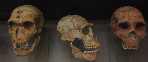
 West‑to‑Baltic Spatial Synopsis
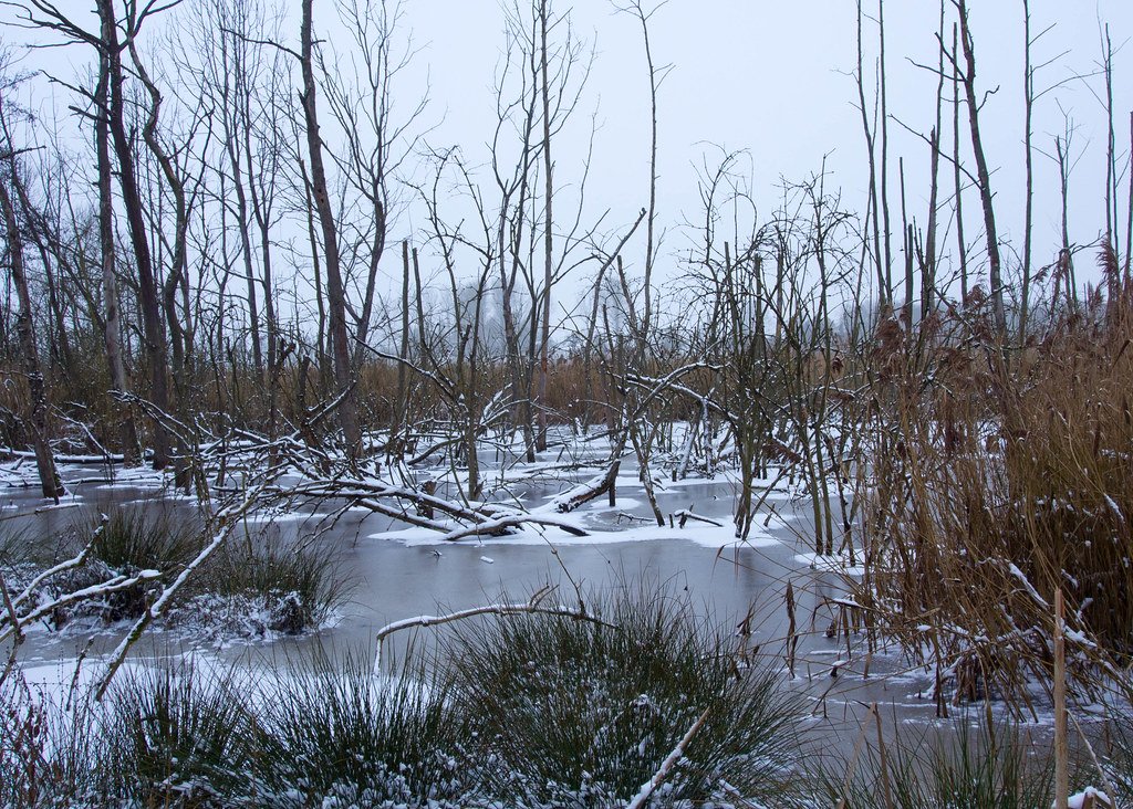 The Cooling Mechanisms
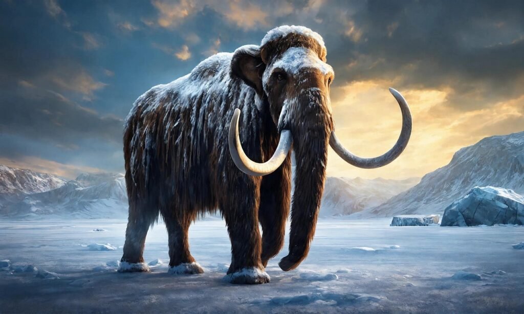 Planet Under Ice — The Consequences of a Colder World
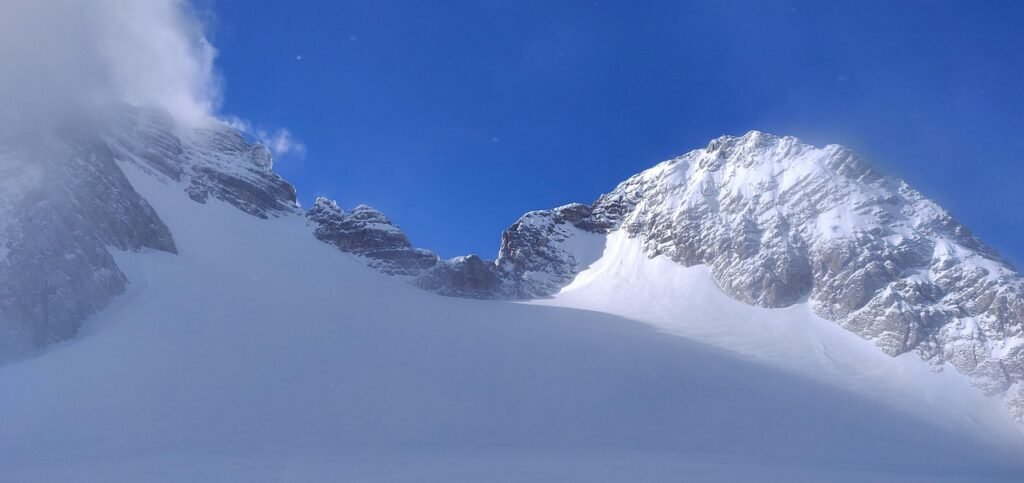 Human Adaptive Solutions


